Seasonal tilt optimization

Playing around with optimizing the tilt of a south-facing adjustable-tilt collector to maximize total insolation capture.

import pvlib
import scipy
import pandas as pd
import numpy as np
import matplotlib.pyplot as plt

for pkg in [pvlib, scipy, pd, np]:
    print(pkg.__name__, pkg.__version__)

pvlib 0.9.0
scipy 1.4.1
pandas 1.3.1
numpy 1.20.3

location = pvlib.location.Location(39.7407, -105.1773, altitude=1790)
# Note: before pvlib 0.9.0 the return values were reversed (meta, tmy = ...)
tmy, meta = pvlib.iotools.get_psm3(location.latitude, location.longitude,
                                   'DEMO_KEY', 'kevin.anderson@nrel.gov',
                                   names='tmy')
reference_year = 2019
tmy.index = [dt.replace(year=reference_year) for dt in tmy.index]

# Note: PSM3 TMYs are already timestamped on the half-hour mark,
# so no need to do a half-interval shift for solar position
solar_position = location.get_solarposition(tmy.index)
dni_extra = pvlib.irradiance.get_extra_radiation(tmy.index)

def simulate_insolation(surface_tilt, solar_position, weather, dni_et):
    poa_components = pvlib.irradiance.get_total_irradiance(
        surface_tilt=surface_tilt,
        surface_azimuth=180,
        solar_zenith=solar_position['apparent_zenith'],
        solar_azimuth=solar_position['azimuth'],
        dni=weather['DNI'],
        ghi=weather['GHI'],
        dhi=weather['DHI'],
        dni_extra=dni_et,
        model='haydavies')
    return poa_components['poa_global'].sum()

Simple tilt optimization

Normal fixed tilt – no seasonal changes

%%time
def objective(tilt):
    # negative so that minimizing is actually maximizing
    return -simulate_insolation(tilt, solar_position, tmy, dni_extra)

# nice and fast!
result = scipy.optimize.minimize_scalar(objective, bounds=[0, 90], method='bounded')
result.x  # optimal tilt in degrees

Wall time: 57.8 ms

37.888115750997976

Partitioned Optimization (anchored, equal widths)

Multiple tilts, equal intervals, first interval starts Jan 1

def optimize_partitioned(n_partitions):
    boundaries = np.linspace(0, 8760, n_partitions+1).astype(int)
    starts = boundaries[:-1]
    ends = boundaries[1:]
    optimal_tilt = pd.Series(np.nan, index=tmy.index)
    for st, ed in zip(starts, ends):
        solpos = solar_position.iloc[st:ed]
        weather = tmy.iloc[st:ed]
        dni_et = dni_extra.iloc[st:ed]
        def objective(tilt):
            return -simulate_insolation(tilt, solpos, weather, dni_et)
        result = scipy.optimize.minimize_scalar(objective, bounds=[0, 90], method='bounded')
        optimal_tilt.iloc[st:ed] = result.x
    return optimal_tilt

tilts = {}
insolations = {}

for n in [1, 4, 12]:
    tilt = optimize_partitioned(n_partitions=n)
    insolation = simulate_insolation(tilt, solar_position, tmy, dni_extra)
    label = f'n={n}'
    tilts[label] = tilt
    insolations[label] = insolation

fig, axes = plt.subplots(1, 2, figsize=(12, 5))
pd.DataFrame(tilts).plot(ax=axes[0])
axes[0].legend(loc='lower right')
axes[0].set_ylim(0, 90)
axes[0].set_ylabel('Optimal Module Tilt [degrees]')

(pd.Series(insolations) / insolations['n=1'] - 1).multiply(100).plot.bar(ax=axes[1])
axes[1].set_ylabel('Insolation Gain over n=1 [%]')

Text(0, 0.5, 'Insolation Gain over n=1 [%]')

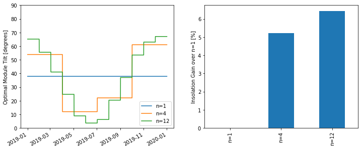
Not a huge increase in total insolation by moving from 4 to 12 adjustments per year. If you add n=2 to this plot it shows hardly any gain over n=1 because this is anchoring at Jan 1 and each 6-month interval has to accommodate both winter and summer and ends up specializing for neither of them. For n=2 it would be better to anchor at e.g. April so that one interval covers late spring to early fall and the other is late fall to early spring so that they can target the respective high and low solar elevations.

Partitioned Optimization (floating, equal widths)

Multiple tilts, equal intervals, starting any time of year (not just Jan 1).

def optimize_partitioned_floating(n_partitions, shift):
    boundaries = shift + np.linspace(0, 8760, n_partitions+1).astype(int)
    starts = boundaries[:-1]
    ends = boundaries[1:]

    # instead of wrapping around, just extend into a duplicate year:
    solar_position2 = pd.concat([solar_position, solar_position])
    tmy2 = pd.concat([tmy, tmy])
    dni_extra2 = pd.concat([dni_extra, dni_extra])
    optimal_tilt = pd.Series(np.nan, index=tmy2.index)

    for st, ed in zip(starts, ends):
        solpos = solar_position2.iloc[st:ed]
        weather = tmy2.iloc[st:ed]
        dni_et = dni_extra2.iloc[st:ed]
        def objective(tilt):
            return -simulate_insolation(tilt, solpos, weather, dni_et)
        result = scipy.optimize.minimize_scalar(objective, bounds=[0, 90], method='bounded')
        optimal_tilt.iloc[st:ed] = result.x
    optimal_tilt = optimal_tilt.dropna()
    optimal_tilt = optimal_tilt.sort_index()
    return optimal_tilt

optimize_partitioned_floating(2, 0).plot()
optimize_partitioned_floating(2, 8760//4).plot()
plt.ylabel('Ideal Tilt [degrees]');

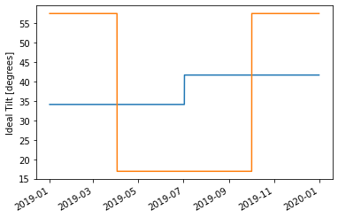
As expected, changing the shift dates so that the n=2 square wave is closer to being in-phase with solar position allows the optimized tilts to be more specialized.

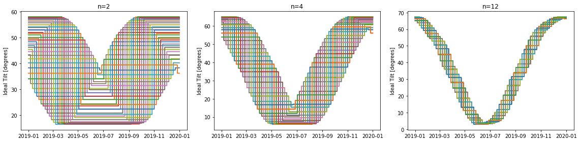
Here is some art showing how the ideal angles change based on anchor choice:

shifts = np.linspace(0, 8760, 73).astype(int)  # 73 evenly divides 365
fig, axes = plt.subplots(1, 3, figsize=(16, 4))
for i, n in enumerate([2, 4, 12]):
    tilts = [optimize_partitioned_floating(n, shift) for shift in shifts]
    axes[i].plot(tmy.index, np.array(tilts).T)
    axes[i].set_ylabel('Ideal Tilt [degrees]')
    axes[i].set_title(f'n={n}')

fig.tight_layout()

Compare annual insolation across n and shift:

for n in [1, 2, 3, 4, 5, 6, 12]:
    insolations = [simulate_insolation(optimize_partitioned_floating(n, shift), solar_position, tmy, dni_extra) for shift in shifts]
    pd.Series(insolations, index=tmy.index[shifts-1]).plot(label=f'n={n}')

plt.legend()
plt.xlabel('Anchor Point')
plt.ylabel('Annual Insolation [Wh/m2]')

equinoxes = pd.to_datetime(['2019-03-20', '2019-09-23'])
for eq in equinoxes:
    plt.axvline(eq, c='grey', ls='--')

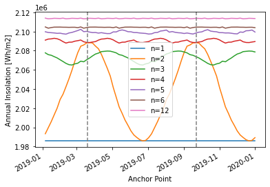
Look at how n=3 performs poorly relative to n=2 for some shifts! I suppose it is mostly down to requiring equal intervals; if nonequal intervals were allowed then annual insolation would presumably be monotonic non-decreasing with n – if n+1 were somehow worse than n, you could just shrink one interval down to zero length and match n exactly.

Also n=2 really isn’t that bad – there’s maybe a ~1% increase from n=2 on the equinox to n=12. And n=4 is no better than equinox-aligned n=2. For n>=4 the shift doesn’t really change the annual insolation capture (though the optimal angles still change for each interval

Note that the code to generate this plot is pretty inefficient for large n; each of these profiles has n periods per year, so there is no new information to be had after 8760/n shifts. E.g. for n=2 a shift of zero is the same as a shift of 4380.

Basic SIMD in Julia   Single-axis tracking: GCR vs max angle