Climate Report

Additional time series data about climate change come in all the time. Here are some plots that I like to track.

I think that what is essential for this problem is a global consciousness,
a view that transcends our exclusive identifications with the generational
and political groupings into which by accident we have been born.

The solution to these problems requires a perspective that embraces the
planet and the future, because we are all in this greenhouse together. 

Carl Sagan, https://youtu.be/Wp-WiNXH6hI?t=985

Keeling Curve (Mauna Loa CO2)

Show code cell source Hide code cell source

import pandas as pd
import numpy as np
import matplotlib.pyplot as plt
import rdtools

plt.rcParams['figure.dpi'] = 100

url = 'https://gml.noaa.gov/webdata/ccgg/trends/co2/co2_weekly_mlo.csv'
df = pd.read_csv(url, skiprows=51, na_values=-999.99)
df.index = pd.to_datetime(df[['year', 'month', 'day']])

ppm_weekly = df['average']
ppm_daily = ppm_weekly.resample('d').interpolate()

_, _, calc_info = rdtools.degradation_year_on_year(ppm_daily)
yoy_changes = calc_info['YoY_values']

moving_avg = ppm_daily.rolling(365, center=True).mean()
ppm_deseasonalized = ppm_daily - moving_avg
grouper = ppm_deseasonalized.groupby(ppm_deseasonalized.index.dayofyear)
median_seasonality = grouper.median()
upper_seasonality = grouper.quantile(0.95)
lower_seasonality = grouper.quantile(0.05)

---------------------------------------------------------------------------
KeyError                                  Traceback (most recent call last)
Input In [1], in <cell line: 10>()
      8 url = 'https://gml.noaa.gov/webdata/ccgg/trends/co2/co2_weekly_mlo.csv'
      9 df = pd.read_csv(url, skiprows=51, na_values=-999.99)
---> 10 df.index = pd.to_datetime(df[['year', 'month', 'day']])
     12 ppm_weekly = df['average']
     13 ppm_daily = ppm_weekly.resample('d').interpolate()

File ~/miniconda3/envs/kevbase-dev/lib/python3.8/site-packages/pandas/core/frame.py:3511, in DataFrame.__getitem__(self, key)
   3509     if is_iterator(key):
   3510         key = list(key)
-> 3511     indexer = self.columns._get_indexer_strict(key, "columns")[1]
   3513 # take() does not accept boolean indexers
   3514 if getattr(indexer, "dtype", None) == bool:

File ~/miniconda3/envs/kevbase-dev/lib/python3.8/site-packages/pandas/core/indexes/base.py:5782, in Index._get_indexer_strict(self, key, axis_name)
   5779 else:
   5780     keyarr, indexer, new_indexer = self._reindex_non_unique(keyarr)
-> 5782 self._raise_if_missing(keyarr, indexer, axis_name)
   5784 keyarr = self.take(indexer)
   5785 if isinstance(key, Index):
   5786     # GH 42790 - Preserve name from an Index

File ~/miniconda3/envs/kevbase-dev/lib/python3.8/site-packages/pandas/core/indexes/base.py:5842, in Index._raise_if_missing(self, key, indexer, axis_name)
   5840     if use_interval_msg:
   5841         key = list(key)
-> 5842     raise KeyError(f"None of [{key}] are in the [{axis_name}]")
   5844 not_found = list(ensure_index(key)[missing_mask.nonzero()[0]].unique())
   5845 raise KeyError(f"{not_found} not in index")

KeyError: "None of [Index(['year', 'month', 'day'], dtype='object')] are in the [columns]"

Show code cell source Hide code cell source

fig, axes = plt.subplots(2, 1, sharex=True, figsize=(6, 6))

# plot this first because it has a shorter index
yoy_changes.plot(ax=axes[1])
yoy_changes.rolling(52, center=True).median().plot(ax=axes[1])
axes[1].set_xlabel(None)
axes[1].set_ylabel('Year-on-year change [%/yr]')
axes[1].grid()

moving_avg.plot(ax=axes[0])
ppm_daily.plot(ax=axes[0])
axes[0].set_ylabel('Dry CO$_2$ Fraction [ppm]')
axes[0].grid()

fig.tight_layout()

---------------------------------------------------------------------------
NameError                                 Traceback (most recent call last)
Input In [2], in <cell line: 4>()
      1 fig, axes = plt.subplots(2, 1, sharex=True, figsize=(6, 6))
      3 # plot this first because it has a shorter index
----> 4 yoy_changes.plot(ax=axes[1])
      5 yoy_changes.rolling(52, center=True).median().plot(ax=axes[1])
      6 axes[1].set_xlabel(None)

NameError: name 'yoy_changes' is not defined

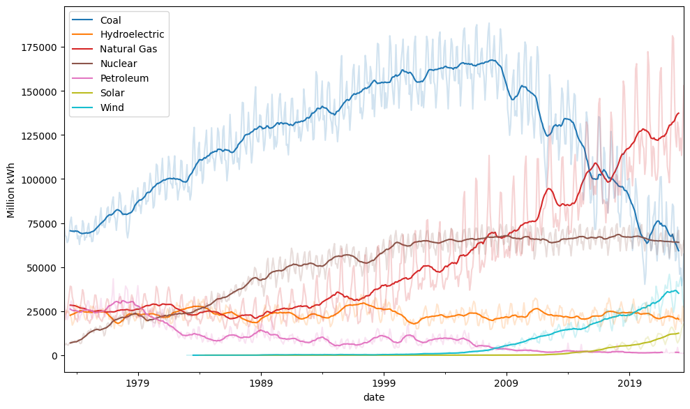
EIA Monthly: Electric Power Sector

Show code cell source Hide code cell source

import pandas as pd
import numpy as np
import matplotlib.pyplot as plt

url = 'https://www.eia.gov/totalenergy/data/browser/csv.php?tbl=T07.02B'
df = pd.read_csv(url)
df = df.loc[~df['Description'].str.contains('Generation Total')]
df = df.loc[~df['YYYYMM'].astype(str).str.endswith('13')]
df['source'] = df['Description'].str.split(",").str[0].str.replace('Electricity Net Generation From ', '')
df['date'] = pd.to_datetime(df['YYYYMM'], format='%Y%m')
df2 = df.pivot(index='date', columns='source', values='Value')
df2 = df2.rename(columns={'Conventional Hydroelectric Power': 'Hydroelectric',
                          'Nuclear Electric Power': 'Nuclear'})
df2 = df2.replace('Not Available', np.nan).replace('Not Meaningful', np.nan).astype(float)
df2 = df2.loc[:, df2.max() > 5000]  # only keep the main players

fractions = 100 * df2.divide(df2.sum(axis=1), axis=0).clip(lower=0)

fig, ax = plt.subplots(figsize=(10, 6))
df2.rolling(12, center=True).mean().plot(ax=ax, colormap='tab10')
ax.legend()
ax.set_ylabel('Million kWh')
fig.tight_layout()
df2.plot(ax=ax, alpha=0.2, colormap='tab10', legend=False)
plt.show()

Show code cell source Hide code cell source

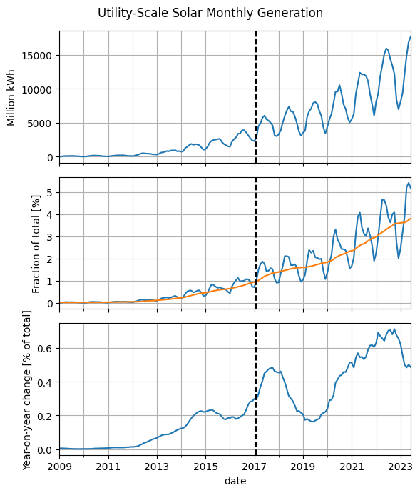
fig, axes = plt.subplots(3, 1, sharex=True, figsize=(6, 7))
fig.suptitle('Utility-Scale Solar Monthly Generation')

df2['Solar'].dropna().loc['2009':].plot(ax=axes[0])
axes[0].set_ylabel('Million kWh')

fractions['Solar'].loc['2009':].plot(ax=axes[1])
moving_average = fractions['Solar'].rolling(12).mean()
moving_average.loc['2009':].plot(ax=axes[1])
axes[1].set_ylabel('Fraction of total [%]')

yoy_change = moving_average - moving_average.shift(12)
yoy_change.loc['2009':].plot(ax=axes[2])
axes[2].set_ylabel('Year-on-year change [% of total]')

for ax in axes:
    ax.axvline('2017-02-01', ls='--', c='k')
    ax.grid(which='both')

fig.tight_layout()

Show code cell source Hide code cell source

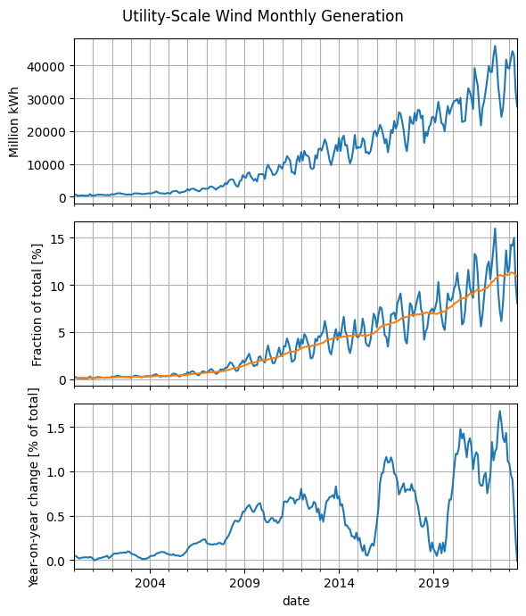
fig, axes = plt.subplots(3, 1, sharex=True, figsize=(6, 7))
fig.suptitle('Utility-Scale Wind Monthly Generation')

df2['Wind'].dropna().loc['2000':].plot(ax=axes[0])
axes[0].set_ylabel('Million kWh')

fractions['Wind'].loc['2000':].plot(ax=axes[1])
moving_average = fractions['Wind'].rolling(12).mean()
moving_average.loc['2000':].plot(ax=axes[1])
axes[1].set_ylabel('Fraction of total [%]')

yoy_change = moving_average - moving_average.shift(12)
yoy_change.loc['2000':].plot(ax=axes[2])
axes[2].set_ylabel('Year-on-year change [% of total]')

for ax in axes:
    ax.grid(which='both')

fig.tight_layout()

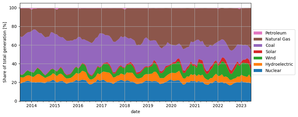
Show code cell source Hide code cell source

# reorder for plotting purposes
col_order = ['Nuclear', 'Hydroelectric', 'Wind', 'Solar',
             'Coal', 'Natural Gas', 'Petroleum']
fractions = fractions[col_order]
fractions.iloc[-12*10:].plot.area(lw=0, figsize=(10, 4))
plt.ylabel('Share of total generation [%]')

handles, labels = plt.gca().get_legend_handles_labels()
plt.legend(reversed(handles), reversed(labels),
           loc='center right', bbox_to_anchor=(1.2, 0.5))
plt.tight_layout()
plt.grid()

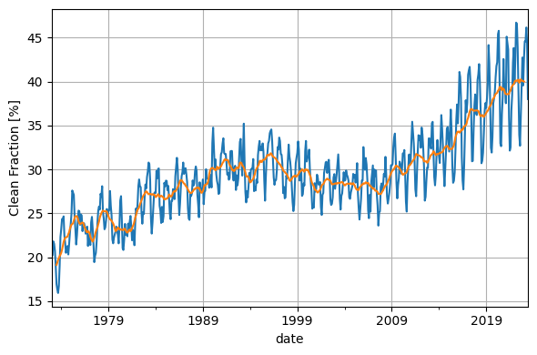
Show code cell source Hide code cell source

clean = ['Solar', 'Wind', 'Hydroelectric', 'Nuclear']
clean_fraction = 100 * df2[clean].sum(axis=1) / df2.sum(axis=1)
clean_fraction.plot()
clean_fraction_rolling = 100 * (
    df2[clean].sum(axis=1).rolling(12, center=True).sum() /
    df2.sum(axis=1).rolling(12, center=True).sum()
)
clean_fraction_rolling.plot()
plt.ylabel('Clean Fraction [%]')
plt.tight_layout()
plt.grid()

Show code cell source Hide code cell source

fractions.assign(clean_fraction=clean_fraction).tail(24)

source	Nuclear	Hydroelectric	Wind	Solar	Coal	Natural Gas	Petroleum	clean_fraction
date
2021-07-01	17.749486	5.672725	5.596148	3.123736	26.059623	41.411726	0.386556	32.142095
2021-08-01	17.582022	5.121672	6.847001	3.009276	25.658286	41.306510	0.475233	32.559971
2021-09-01	19.471349	5.108749	8.744410	3.363259	23.656471	39.193898	0.461864	36.687767
2021-10-01	19.225829	5.609387	10.597540	3.032225	20.451449	40.595974	0.487596	38.464981
2021-11-01	21.074837	6.472696	11.997935	2.601607	19.124287	38.191189	0.537449	42.147075
2021-12-01	22.124844	7.342375	12.457838	1.894092	18.635210	37.079001	0.466641	43.819148
2022-01-01	19.648130	7.266734	10.593376	2.258741	24.220136	35.052329	0.960554	39.766981
2022-02-01	19.882530	7.330795	12.200840	2.979657	22.598647	34.503456	0.504076	42.393822
2022-03-01	20.599277	8.234918	14.019994	3.854628	19.652440	33.638743	NaN	46.708817
2022-04-01	19.213153	6.768627	15.960220	4.651368	18.971811	34.024399	0.410424	46.593367
2022-05-01	19.454481	7.049620	12.781013	4.635027	18.948576	36.684719	0.446564	43.920141
2022-06-01	18.046523	7.355952	9.188972	4.380111	19.992738	40.621075	0.414628	38.971559
2022-07-01	16.943656	5.930102	7.205831	3.849752	21.104321	44.618513	0.347826	33.929341
2022-08-01	17.434188	5.469584	6.159135	3.629690	21.380218	45.543385	0.383801	32.692597
2022-09-01	19.037261	4.997759	8.069551	4.005375	19.227136	44.200185	0.462733	36.109945
2022-10-01	19.764535	4.883314	10.998682	4.079339	17.986522	41.785433	0.502176	39.725870
2022-11-01	20.248213	6.095464	13.640923	2.750624	18.196231	38.581512	0.487033	42.735224
2022-12-01	19.936510	6.280340	11.326968	2.015887	20.977570	38.183218	1.279508	39.559705
2023-01-01	21.435912	6.909181	11.811051	2.444816	18.054992	38.964551	0.379497	42.600961
2023-02-01	20.631132	6.529218	14.245167	3.163071	15.583960	39.386561	0.460890	44.568589
2023-03-01	20.023073	6.543128	14.127610	3.886425	15.770735	39.273379	0.375649	44.580236
2023-04-01	19.751619	6.233706	14.969008	5.202725	13.810082	39.632281	0.400578	46.157059
2023-05-01	19.688290	8.928018	10.254452	5.412216	13.857508	41.507467	0.352050	44.282975
2023-06-01	19.045293	5.733255	8.047143	5.180946	16.820428	44.835486	0.337448	38.006638

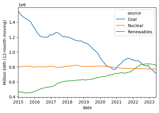
Show code cell source Hide code cell source

rolling = df2.rolling(12).sum()
rolling['Renewables'] = rolling[['Solar', 'Wind', 'Hydroelectric']].sum(axis=1)
rolling.loc['2015':, ['Coal', 'Nuclear', 'Renewables']].plot()
plt.ylabel('Million kWh (12-month moving)');

This page was last regenerated on:

Show code cell source Hide code cell source

import datetime
datetime.date.today().strftime('%Y-%m-%d')

previous

Blog