OpenGL Compute Shaders: First Steps
This notebook is a first exploration into general-purpose GPU (GPGPU) computing using OpenGL’s compute shaders. OpenGL is primarily geared towards rendering graphics and most of its functionality is organized into a sequential rendering pipeline. However, it also includes the ability to run computations outside of the rendering pipeline using so-called “compute shaders”. In essence, a shader is just a little program, written in a C-like language, that executes on the GPU. I am neither qualified nor interested in explaining more than that; if you’re interested then I suggest reading one of the many OpenGL tutorials on the internet. I warn you in advance: it is a big rabbit hole!
If the goal is general-purpose GPU computing, you might wonder why I chose to use OpenGL (geared towards graphics, with GPGPU as an auxiliary function) instead of something like CUDA or OpenCL. I have the naive impression that OpenGL is easier to set up on a new computer than the the more general alternatives are, and a long-term goal of mine is to distribute GPU-accelerated code to the masses, so ease of installation is important. Perhaps someday I’ll change my mind and switch to OpenCL, but for now I experiment with OpenGL.
This is my first foray into the world of GPU programming, so I don’t necessarily suggest using this as learning material. I can’t promise I’m following best practices because I don’t know what the best practices are. This is just a record of what I managed to get working.
Currently I’m using moderngl as an OpenGL interface to my graphics card:
!python -m moderngl
moderngl 5.6.4
--------------
vendor: AMD
renderer: AMD RENOIR (LLVM 13.0.1, DRM 3.44, 5.16.19-76051619-generic)
version: 4.6 (Core Profile) Mesa 22.0.1
python: 3.8.13 (default, Mar 28 2022, 11:38:47)
[GCC 7.5.0]
platform: linux
code: 460
import moderngl
import numpy as np
import pandas as pd
import matplotlib.pyplot as plt
import time

plt.rcParams['figure.dpi'] = 100
The overall strategy here is more or less to set up an OpenGL context, transfer the computation inputs to the GPU, perform the computation, and transfer the computation outputs back to the CPU.
Here is a small helper function that takes some generic computation and an input array, and handles all the OpenGL setup and data shuffling to and from the GPU. This is probably a dumb way to use OpenGL but I wanted an easy way to compare different computations, so this is what I used. I use 32-bit floats because I’m told that’s what GPUs prefer. Future applications might require switching from single-precision to double-precision floats.
# create a single OpenGL context and re-use it for all that follows
context = moderngl.create_standalone_context(require=430)


def compute(job, inputs, groupsize=1024):
    """
    Helper function to run a computation on some input array.
    """

    N = len(inputs)

    SHADER_SOURCE = ("""
    #version 430

    #define GROUPSIZE %%N%%

    layout(local_size_x=GROUPSIZE, local_size_y=1, local_size_z=1) in;

    layout (std430, binding=0) buffer in_0
    {
        float inputs[1];
    };

    layout (std430, binding=1) buffer out_0
    {
        float outputs[1];
    };

    void main()
    {
        // setup
        const int local_id = int(gl_LocalInvocationID.x);
        const int group_id = int(gl_WorkGroupID.x);
        const int i = group_id * GROUPSIZE + local_id;
        // custom job, to be specified externally while I experiment
        %%JOB%%
    }
    """
    .replace("%%N%%", str(min(len(inputs), groupsize)))
    .replace("%%JOB%%", job)
    )

    compute_shader = context.compute_shader(SHADER_SOURCE)

    buffer_inputs = context.buffer(inputs)
    buffer_outputs = context.buffer(reserve=inputs.nbytes)

    buffer_inputs.bind_to_storage_buffer(0)
    buffer_outputs.bind_to_storage_buffer(1)

    n_group = 1 + (len(inputs)-1) // groupsize
    compute_shader.run(group_x=n_group)

    outputs = np.frombuffer(buffer_outputs.read(), dtype=np.float32)
    return outputs
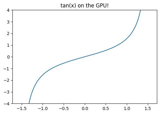
We can try it out on a simple example:
inputs = np.linspace(-np.pi/2 + 0.01, np.pi/2 - 0.01, num=1000, dtype='f4')
computation = "outputs[i] = tan(inputs[i]);"
outputs = compute(computation, inputs)

plt.plot(inputs, outputs)
plt.ylim(-4, 4)
plt.title('tan(x) on the GPU!')
Text(0.5, 1.0, 'tan(x) on the GPU!')
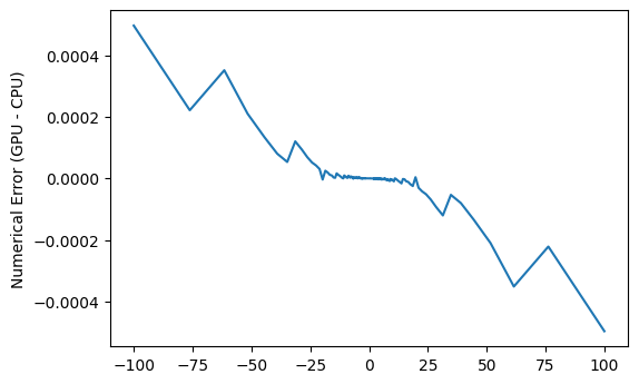
One important thing to be aware of is that IEEE-754 compliance is apparently not guaranteed (or I’m doing something wrong):
outputs_cpu = np.tan(inputs)
plt.plot(outputs_cpu, outputs - outputs_cpu)
plt.ylabel('Numerical Error (GPU - CPU)')
Text(0, 0.5, 'Numerical Error (GPU - CPU)')
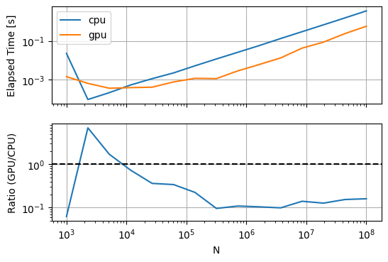
Now let’s take a look at speed. Shuffling data between CPU and GPU isn’t free. The question is how much overhead that introduces, and what conditions are necessary for using the GPU to be worthwhile. First up let’s look at how arctan(x) runtime scales with the size of x. For the CPU runtimes I’m calling numpy – perhaps using numba would be a fairer comparison, but I’m just feeling things out at this point.
def timing_plots(timings):
    timings = pd.DataFrame(timings).set_index('N')
    fig, axes = plt.subplots(2, 1, sharex=True)
    timings.plot(ax=axes[0], logx=True, logy=True)
    axes[0].set_ylabel('Elapsed Time [s]')
    axes[0].grid()
    ratio = timings['gpu'] / timings['cpu']
    ratio.plot(ax=axes[1], logy=True)
    axes[1].axhline(1, ls='--', c='k')
    axes[1].set_ylabel('Ratio (GPU/CPU)')
    axes[1].grid()
N = np.logspace(3, 8, num=15).astype(int)

timings = []

for n in N:
    x = np.linspace(0, 1, num=n, dtype='f4')
    timing = {'N': n}

    st = time.perf_counter()
    _ = np.arctan(x)
    ed = time.perf_counter()
    timing['cpu'] = ed - st

    st = time.perf_counter()
    _ = compute("outputs[i] = atan(inputs[i]);", x)
    ed = time.perf_counter()
    timing['gpu'] = ed - st

    timings.append(timing)

timing_plots(timings)
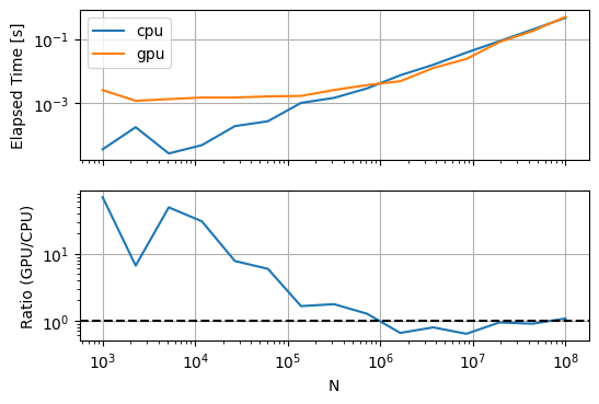
So it seems like for this problem (arctan(x)) the improved scaling ability on the GPU doesn’t really result in a meaningful improvement, even for large input sizes. However, input size isn’t the only variable here – what about problem complexity? Input size is probably the main influence on the overhead cost (since it directly affects how much data you’re sending to/from the GPU), so let’s use the same sizes but increase the computation cost by 10x:
timings = []

for n in N:
    x = np.linspace(0, 1, num=n, dtype='f4')
    timing = {'N': n}

    st = time.perf_counter()
    _ = np.arctan(np.arctan(np.arctan(
        np.arctan(np.arctan(np.arctan(
        np.arctan(np.arctan(np.arctan(np.arctan(x))))))))))
    ed = time.perf_counter()
    timing['cpu'] = ed - st

    st = time.perf_counter()
    _ = compute("outputs[i] = atan(atan(atan(atan(atan(atan(atan(atan(atan(atan(inputs[i]))))))))));", x)
    ed = time.perf_counter()
    timing['gpu'] = ed - st

    timings.append(timing)

timing_plots(timings)
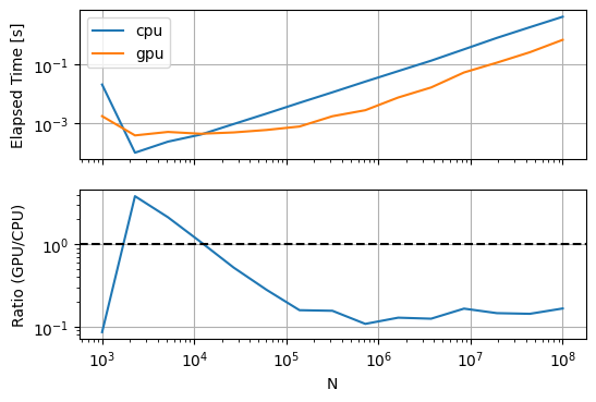
Now we see that the GPU starts winning at relatively small input sizes around 1e4! But wait a minute, isn’t the CPU-based method unfairly penalized because of repeated and unnecessary memory allocations? Let’s fix that by using numpy’s out kwarg:
timings = []

for n in N:
    x = np.linspace(0, 1, num=n, dtype='f4')
    timing = {'N': n}

    x1 = np.empty_like(x)
    st = time.perf_counter()
    np.arctan(x, out=x1)
    for _ in range(9):
        np.arctan(x1, out=x1)
    ed = time.perf_counter()
    timing['cpu'] = ed - st

    st = time.perf_counter()
    _ = compute("""
    float y = atan(inputs[i]);
    for(int i = 0; i < 9; i++){
        y = atan(y);
    }
    outputs[i] = y;
    """, x)
    ed = time.perf_counter()
    timing['gpu'] = ed - st

    timings.append(timing)

timing_plots(timings)
Doesn’t seem to have really changed the picture, so maybe we don’t need to stress out about memory allocations in this context.
Let’s bump up the complexity again, this time to 100 arctans:
timings = []

for n in N:
    x = np.linspace(0, 1, num=n, dtype='f4')
    timing = {'N': n}

    x1 = np.empty_like(x)
    st = time.perf_counter()
    np.arctan(x, out=x1)
    for _ in range(99):
        np.arctan(x1, out=x1)
    ed = time.perf_counter()
    timing['cpu'] = ed - st

    st = time.perf_counter()
    _ = compute("""
    float y = atan(inputs[i]);
    for(int i = 0; i < 99; i++){
        y = atan(y);
    }
    outputs[i] = y;
    """, x)
    ed = time.perf_counter()
    timing['gpu'] = ed - st

    timings.append(timing)

timing_plots(timings)
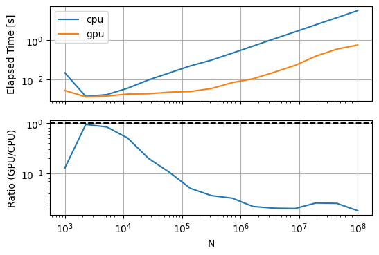
Now the GPU wins at basically all problem sizes, but with massive speedup for medium-large problems!
Let’s disect our OpenGL code and see what the line-by-line runtime looks like:
inputs = x = np.linspace(0, 1, num=10**5, dtype='f4')
groupsize = 1024
job = """
float y = atan(inputs[i]);
for(int i = 0; i < 99; i++){
    y = atan(y);
}
outputs[i] = y;
"""

n_group = 1 + (len(inputs)-1) // groupsize

st = time.perf_counter()
SHADER_SOURCE = ("""
#version 430

#define GROUPSIZE %%N%%

layout(local_size_x=GROUPSIZE, local_size_y=1, local_size_z=1) in;

layout (std430, binding=0) buffer in_0
{
    float inputs[1];
};

layout (std430, binding=1) buffer out_0
{
    float outputs[1];
};

void main()
{
    // setup
    const int local_id = int(gl_LocalInvocationID.x);
    const int group_id = int(gl_WorkGroupID.x);
    const int i = group_id * GROUPSIZE + local_id;
    // custom job, to be specified externally while I experiment
    %%JOB%%
}
"""
.replace("%%N%%", str(min(len(inputs), groupsize)))
.replace("%%JOB%%", job)
)
ed = time.perf_counter()
print('shader definition & interpolation:', ed - st)

st = time.perf_counter()
compute_shader = context.compute_shader(SHADER_SOURCE)
ed = time.perf_counter()
print('shader compilation:', ed - st)

st = time.perf_counter()
buffer_inputs = context.buffer(inputs)
buffer_outputs = context.buffer(reserve=inputs.nbytes)
ed = time.perf_counter()
print('buffer initialization:', ed - st)

st = time.perf_counter()
buffer_inputs.bind_to_storage_buffer(0)
buffer_outputs.bind_to_storage_buffer(1)
ed = time.perf_counter()
print('buffer binding:', ed - st)

st = time.perf_counter()
compute_shader.run(group_x=n_group)
ed = time.perf_counter()
print('shader execution:', ed - st)

st = time.perf_counter()
outputs = np.frombuffer(buffer_outputs.read(), dtype=np.float32)
ed = time.perf_counter()
print('fetching results:', ed - st)
shader definition & interpolation: 4.4764019548892975e-05
shader compilation: 0.0005510500050149858
buffer initialization: 0.001609519007615745
buffer binding: 6.838899571448565e-05
shader execution: 4.4234038796275854e-05
fetching results: 0.002403047983534634
I’m not 100% sure whether all of the actual computation is correctly binned here – it could be that some of the time currently allocated to “fetching results” is actually just idle time waiting for the GPU to finish its computations.
Regardless, all of this is just mind-bogglingly fast. My main conclusion is that, especially for medium-large inputs (>1e4) and complex computations, all-in GPU runtime (including data transfer) can be significantly (1-2 orders of magnitude) faster than the CPU runtime, suggesting that even with my inexperienced and likely inefficient use of OpenGL it is a viable option for speeding up real-world computations.