Summing Uniform Distributions

The distribution of the sum of N uniformly distributed variables came up in a recent RdTools PR. The approach taken there was to just sample each distribution and sum the samples, but I wondered how it could be done analytically. This notebook is inspired by this StackExchange post and extends the derivation from just summing two uniform distributions on \([0,1]\) to two distributions with arbitrary bounds.

Given two independent random variables \(A\) and \(B\) with probability densities \(f_a(x)\) and \(f_b(x)\), the probability density \(f_c(x)\) of their sum \(A + B = C\) is given by the convolution \(f_a * f_b\):

\[ f_c(x) = \int_{-\infty}^{\infty} f_a(x') f_b(x - x') \mathrm{d}x' \]

For the case where \(A\) and \(B\) are uniformly distributed, we have:

\[\begin{split} f_a(x) = \begin{cases} \frac{1}{a_2 - a_1} & a_1 \le x \le a_2 \\ 0 & \mathrm{otherwise} \end{cases} \end{split}\]

\[\begin{split} f_b(x) = \begin{cases} \frac{1}{b_2 - b_1} & b_1 \le x \le b_2 \\ 0 & \mathrm{otherwise} \end{cases} \end{split}\]

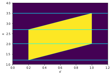
Using these definitions, let’s visualize in the \(X'-X\) plane where the integrand is nonzero:

import matplotlib.pyplot as plt
import numpy as np

a1 = 0.2
a2 = 1.0
b1 = 1.0
b2 = 2.5

Xlim = [1, 4]
Xplim = [0, 1.2]
Xp, X = np.meshgrid(np.linspace(*Xplim, 1000), np.linspace(*Xlim, 1000))
nonzero = (a1 <= Xp) & (Xp <= a2) & (b1 <= X - Xp) & (X - Xp <= b2)

plt.imshow(nonzero, extent=Xplim + Xlim, aspect='auto', origin='lower')
plt.xlabel("x'")
plt.ylabel("x")

plt.axhline(b1 + a1, c='cyan')
plt.axhline(b1 + a2, c='cyan')
plt.axhline(b2 + a1, c='cyan')
plt.axhline(b2 + a2, c='cyan');

The cross-section of the parallelogram is the range of \(x'\) where the integrand is nonzero, so the lower and upper bounds of each cross-section define the limits of integration as a function of \(x\). Notice that it can be divided into three domains with nonzero probability, drawn here separated by the cyan lines. Going up from the bottom, they are defined by:

Domain	Domain bounds	Integration bounds
1	\(b_1 + a_1 \le x \le b_1 + a_2\)	\(a_1 \le x' \le x - b_1\)
2	\(b_1 + a_2 \le x \le b_2 + a_1\)	\(a_1 \le x' \le a_2\)
3	\(b_2 + a_1 \le x \le b_2 + a_2\)	\(x - b_2 \le x' \le a_2\)

Finally, note that with the restricted bounds of integration \(x_1\) and \(x_2\), the integrand becomes the constant \((a_2-a_1)^{-1}(b_2-b_1)^{-1}\) and so the integral simplifies:

\[\begin{split} \begin{align} f_c(x) &= \frac{1}{(a_2-a_1)(b_2-b_1)} \int_{x'_1}^{x'_2} \mathrm{d}x' \\ &= \frac{x'_2 - x'_1}{(a_2-a_1)(b_2-b_1)} \end{align} \end{split}\]

where \(x'_1\) and \(x'_2\) are given by the integration bounds in the above table as a function of \(x\).

Note that we have assumed \(b_1 + a_2 \le b_2 + a_1\). If that is not the case, swap the \(a\)s and \(b\)s.

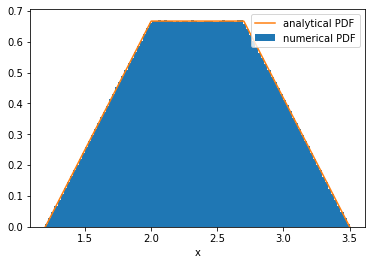
# Numerical approach
N = 10000000
A = np.random.uniform(a1, a2, N)
bd = 1/(b2-b1)
B = np.random.uniform(b1, b2, N)
C = A + B

plt.hist(C, bins=100, density=True, label='numerical PDF')


# Analytical approach
scale = 1/(a2-a1)/(b2-b1)

def f_c(x, a1, a2, b1, b2):
    if a1 + b2 < b1 + a2:
        a1, a2, b1, b2 = b1, b2, a1, a2

    y = np.zeros_like(x)
    region1 = (b1 + a1 <= x) & (x <= b1 + a2)
    region2 = (b1 + a2 <= x) & (x <= b2 + a1)
    region3 = (b2 + a1 <= x) & (x <= b2 + a2)
    y[region1] = scale * (x[region1] - b1 - a1)
    y[region2] = scale * (a2 - a1)
    y[region3] = scale * (a2 - (x[region3] - b2))
    return y

x = np.linspace(a1+b1, a2+b2, 1000)
y = f_c(x, a1, a2, b1, b2)
plt.plot(x, y, label='analytical PDF')
plt.xlabel('x')
plt.legend();

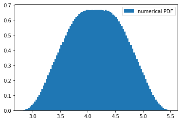
Going back to the original problem of summing not just two random variables but \(N\) of them, it seems reasonable to expect that increasing \(N\) will increase the order of the polynomials involved, and visualizing it for \(N=3\) does show some higher-order behavior:

A = np.random.uniform(a1, a2, N)
bd = 1/(b2-b1)
B = np.random.uniform(b1, b2, N)
C = np.random.uniform(1.6, 2.0, N)
D = A + B + C

plt.hist(D, bins=100, density=True, label='numerical PDF')
plt.legend();

Modeling copper losses in a boost converter   Floating Point Fun