Floating Point Fun

Computers must represent real numbers with some finite precision (ignoring symbolic algebra packages), and sometimes that precision limit ends up causing problems that you might not expect. Here are a couple examples.

exp and expm1

The function \(f(x) = \exp(x) - 1\) is kind of fun – by subtracting one from the exponential, it removes the only constant term in the Maclaurin series of \(\exp(x)\):

\[\exp(x) = \sum_{n=0}^\infty \frac{x^n}{n!} = 1 + x + \frac{x^2}{2} + \frac{x^3}{6} + \, ...\]

And so by subtracting off one, only terms that depend on \(x\) are left:

\[\exp(x) - 1 = \sum_{n=1}^\infty \frac{x^n}{n!} = x + \frac{x^2}{2} + \frac{x^3}{6} + \, ...\]

Notice that, for positive \(x \ll 1\), the series can be approximated with just \(\exp(x) - 1 \approx x\), with the approximation improving as \(x\) approaches zero. A similar argument lets us approximate \(\exp(x)\) as \(1+x\), again for positive \(x \ll 1\).

Using floating point math to perform such calculations is tricky because of the finite amount of precision available to represent real numbers. For example evaluating \(\exp(2^{-100})\) should return some number close to \(1 + 2^{-100}\), meaning we’d need 100 bits of significand precision to be able to distinguish the result from 1. The standard floating point type used by most computers is the double-precision float, which uses 64 bits, of which 52 are used for significand precision. This is easy to demonstrate:

In [1]: 1 + 2**-52 > 1
Out[1]: True

In [2]: 1 + 2**-53 > 1
Out[2]: False

This precision limit means that, although the true value of \(\exp(2^{-53}) - 1\) requires only a few bits of significand precision to represent, we must take care to not exceed our precision limits in the intermediate calculations. So calculating \(\exp(2^{-53})\) first and then subtracting off 1 is not going to work because by “wasting” all of our precision storing the 1 in \(1 + 2^{-53}\), we’re losing digits farther down – they get rounded off. In code:

In [3]: import numpy as np

In [4]: np.exp(2**-53) - 1
Out[4]: np.float64(0.0)

In [5]: np.exp(2**-52) - 1
Out[5]: np.float64(2.220446049250313e-16)

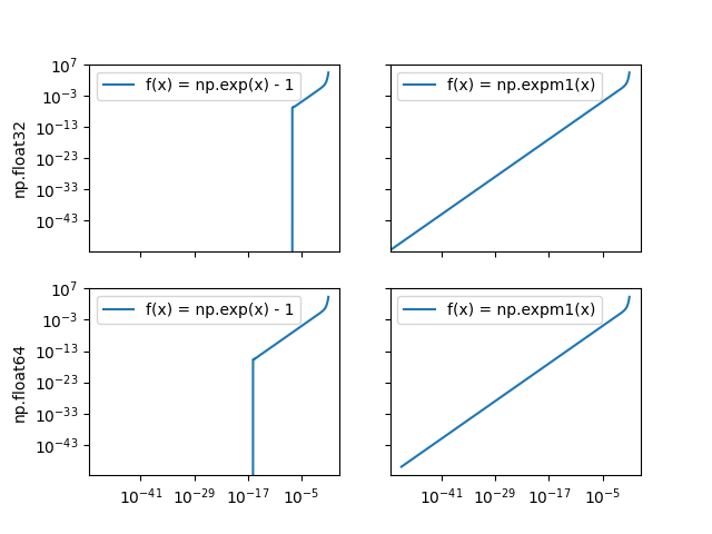
Luckily some smart folks have worked around this and provided us with functions like np.expm1 that are cleverly written to avoid wasting precision in the intermediate calculations. So let’s see how it performs against the naive method, trying out two floating point formats: the double-precision format described above and the single-precision format that uses only 32 bits (23 used for significand). For reference, these bit widths give us about 16 and 7 digits of accuracy (\(2^{-52}\approx 2 \times 10^{-16}\); \(2^{-23}\approx 1 \times 10^{-7}\)). Recall that, for small \(x\), the true value of \(\exp(x) - 1\) should be close to \(x\), meaning the values should follow the \(1:1\) line for \(x \ll 10^{0}\).

In [6]: import matplotlib.pyplot as plt

In [7]: fig, axes = plt.subplots(2, 2, sharex=True, sharey=True)

In [8]: for j, dtype in enumerate([np.float32, np.float64]):
   ...:     x = np.logspace(-50, 1, num=500, dtype=dtype)
   ...:     cases = {
   ...:         'f(x) = np.exp(x) - 1': np.exp(x) - 1,
   ...:         'f(x) = np.expm1(x)': np.expm1(x),
   ...:     }
   ...:     for i, (label, y) in enumerate(cases.items()):
   ...:         axes[j, i].loglog(x, y, label=label)
   ...:         axes[j, i].legend(loc='upper left')
   ...: 

In [9]: axes[0, 0].set_ylabel('np.float32'); axes[1, 0].set_ylabel('np.float64');

In [10]: plt.show()

So the naive method fails once \(x\) crosses the datatype precision limit, but the mathemagics baked into np.expm1 return the right answer across the full domain.

aoi out of bounds

Round-off error showed up recently in a pvlib issue. The angle of incidence (AOI) projection is a measure of how well-aligned a solar panel is with the sun’s position in the sky and is calculated with:

In [11]: def aoi_projection(surface_tilt, surface_azimuth, solar_zenith, solar_azimuth):
   ....:     return (
   ....:         np.cos(surface_tilt) * np.cos(solar_zenith) +
   ....:         np.sin(surface_tilt) * np.sin(solar_zenith) *
   ....:         np.cos(solar_azimuth - surface_azimuth)
   ....:     )
   ....: 

Mathematically this is the dot product between the solar position unit vector and the solar panel normal, and as such is bounded in the interval \([-1, +1]\).

Consider the case where the panel is perfectly aligned with the sun, i.e. surface_tilt==solar_zenith and surface_azimuth==solar_azimuth. Then the calculation, barring any precision issues, should return exactly 1. However, for certain input values, round-off in the intermediate steps end up returning “impossible” values slightly greater than 1:

In [12]: zenith = np.radians(89.26778228223463)

In [13]: azimuth = np.radians(60.932028605997004)

In [14]: aoi_projection(zenith, azimuth, zenith, azimuth)
Out[14]: np.float64(1.0000000000000002)

Because the typical next step is to calculate the angle of incidence itself with \(\theta_{aoi} = \cos^{-1}(\textrm{projection})\), that very small error is actually kind of a big deal because it pushes projection out of the domain of \(\cos^{-1}\), meaning any downstream calculations get polluted with NaN:

In [15]: np.arccos(aoi_projection(zenith, azimuth, zenith, azimuth))
Out[15]: np.float64(nan)

Summing Uniform Distributions   T_cell_typ_avg