Basic SIMD in Julia#
This post summarizes what I’ve learned from a few places on the web (mostly Wikipedia and this thread on the Julia Discourse). I am indebted to countless people in the open-source community and Chris Elrod’s posts in that thread are a stand-out example.
SIMD (single instruction, multiple data) is a cool feature of modern CPUs that allows more than one value to be operated on in a single instruction. This is sort of “closer to the metal” than traditional parallel processing techniques (multiprocessing, multithreading) in that the OS doesn’t have a role in making it happen – it’s just a special type of CPU instruction. As a simple example, a CPU capable of 64-bit SIMD could load two 32-bit ints at once and apply some operation to both of them, instead of loading and operating on them one at a time.
Apparently recent Intel CPUs are capable of 512-bit SIMD. Mine is not so recent and supports a more limited form (256-bit, among other restrictions). Check out this list of CPU flags, which includes a bunch of gibberish that is over my head (here’s a guide if you’re interested), but notice things like sse, sse2, and avx.
print(readchomp(pipeline(`cat /proc/cpuinfo`, `grep flags`, `head -n 1`)))
flags : fpu vme de pse tsc msr pae mce cx8 apic sep mtrr pge mca cmov pat pse36 clflush dts acpi mmx fxsr sse sse2 ss ht tm pbe syscall nx rdtscp lm constant_tsc arch_perfmon pebs bts rep_good nopl xtopology nonstop_tsc cpuid aperfmperf pni pclmulqdq dtes64 monitor ds_cpl vmx smx est tm2 ssse3 cx16 xtpr pdcm pcid sse4_1 sse4_2 x2apic popcnt tsc_deadline_timer aes xsave avx f16c rdrand lahf_lm cpuid_fault epb pti tpr_shadow vnmi flexpriority ept vpid fsgsbase smep erms xsaveopt dtherm ida arat pln pts
AVX is the most capable of the three and allows 256-bit operations, so my CPU (Sandy-Bridge era i5) can operate on four double-precision floats at a time (4 doubles multiplied by 64 bits per double = 256 bits).
Julia’s LoopVectorization package purports to make it trivial to enable SIMD on a naive loop using the hilariously-named @turbo macro. I don’t have any clue how it works under the hood. But let’s see if it actually helps performance on some simple calculations, and in particular compare it with the @simd macro included in base Julia.
Benchmarking things accurately is tricky in any language. In Julia a big gotcha is making sure you’re not including compilation time. The BenchmarkTools packages provides a fancy @btime and @benchmark macros to help with this. I also want to see how the benchmarks change with array size, because look at this amazing chart in the LoopVectorization docs: https://juliasimd.github.io/LoopVectorization.jl/latest/examples/dot_product/
I’m curious what pattern my computer will show, if anything. Maybe BenchmarkTools would iterate across input sizes for me if I actually read the docs for once, but what’s the harm in reinventing the wheel?
using LoopVectorization: @turbo
using BenchmarkTools: @benchmark
using CairoMakie: Figure, Axis, Legend, lines!
using Statistics: median
As Chris pointed out in the thread linked above, Julia’s logic for detecting good functions to automatically inline does not give the weight to otherwise simple functions that use @turbo. So to make the comparison fair (i.e. prevent some, but not all, functions from benefiting from inlining), we’ll manually @inline everything. Otherwise the @turbo variant would lag behind the other accelerated variants.
The first experiment tests the performance of a simple element-wise multiplication function:
# an uninspired first test -- element-wise multiplication
@inline function vmul!(a, b, c)
    for i in eachindex(a)
        c[i] = a[i] * b[i]
    end
end

# same as above, but using @turbo
@inline function vmul_turbo!(a, b, c)
    @turbo for i in eachindex(a)
        c[i] = a[i] * b[i]
    end
end

# same, but with @inbounds for comparison
@inline function vmul_inbounds!(a, b, c)
    @inbounds for i in eachindex(a)
        c[i] = a[i] * b[i]
    end
end

# same, but with @inbounds and @simd for comparison
@inline function vmul_inbounds_simd!(a, b, c)
    @inbounds @simd for i in eachindex(a)
        c[i] = a[i] * b[i]
    end
end

# to show function call penalty
@noinline function vmul_turbo_noinline!(a, b, c)
    @turbo for i in eachindex(a)
        c[i] = a[i] * b[i]
    end
end
vmul_turbo_noinline! (generic function with 1 method)
Now, a simple helper function to iterate over array sizes and accumulate timings. We choose the minimum as the summary statistic following this paper:
Chen, Jiahao and Jarrett Revels. “Robust benchmarking in noisy environments.” ArXiv abs/1608.04295 (2016).
function get_times(func, N)
    times = Float64[]
    for n in N
        a = rand(n)
        b = rand(n)
        c = similar(a)
        bench = @benchmark $func($a, $b, $c)
        push!(times, minimum(bench.times))
    end
    return times
end
get_times (generic function with 1 method)
N = range(32, 128, step=1)

times1 = get_times(vmul!, N)
times2 = get_times(vmul_turbo!, N)
times3 = get_times(vmul_inbounds!, N)
times4 = get_times(vmul_inbounds_simd!, N)
times5 = get_times(vmul_turbo_noinline!, N);
fig = Figure(resolution = (1000,500))
ax = Axis(fig[1, 1], xlabel="N", ylabel="GFLOPS")

l1 = lines!(ax, N, N ./ times1)
l2 = lines!(ax, N, N ./ times2)
l3 = lines!(ax, N, N ./ times3)
l4 = lines!(ax, N, N ./ times4)
l5 = lines!(ax, N, N ./ times5)

fig[1, 2] = Legend(fig, [l1, l2, l3, l4, l5], ["Baseline", "@turbo", "@inbounds", "@inbounds @simd", "@turbo @noinline"])

display(fig)

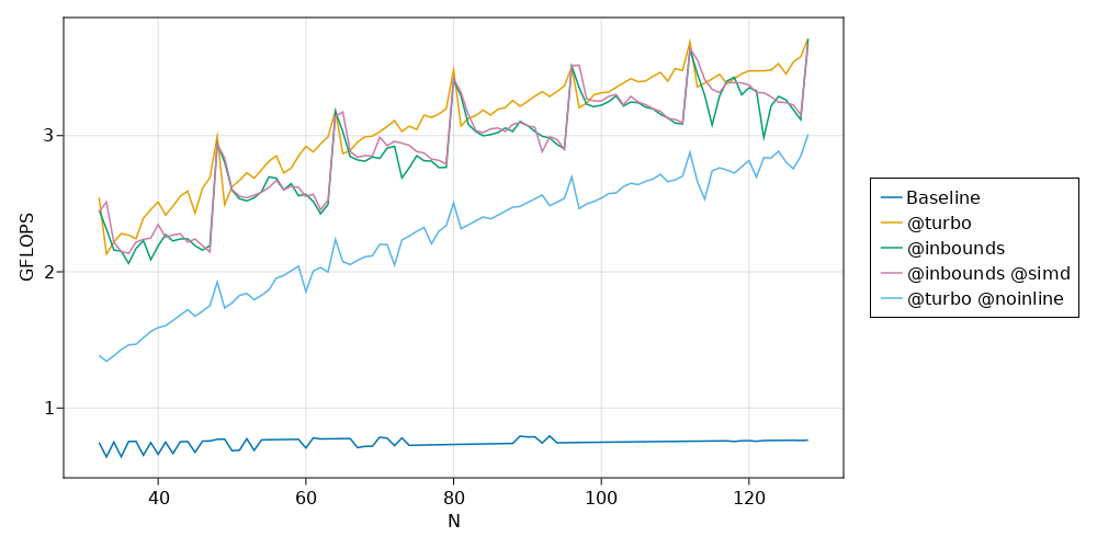
Notice a few things here:
There’s no real performance difference between
@inboundsand@inbounds @simd. This (as Chris pointed out) is because Julia automatically detects cases where floating point associativity issues don’t prevent automatic reordering of operations and applies@simdautomatically. Order doesn’t matter (in a floating point sense) for element-wise multiplication, so Julia automatically applies@simdwithout us asking it to.@turbooffers more consistent performance, partially avoiding the rough sawtooth profile shown by@simd. This has to do with doing a better job of optimizing the remainder of an array after all the complete SIMD-able chunks are processed. The LoopVectorization docs go into detail here. Chris tells me that LoopVectorization can’t do as good a job on handling the remainder on this older CPU, and so the performance for \(N \bmod 16 \neq 0\) is worse than it would be on a newer CPU.
So let’s try something where order does matter in a floating point sense. The LoopVectorization docs use the dot product, so let’s do the same:
# something that can't be freely reassociated -- the dot product
@inline function dot_product(a, b)
    dp = zero(eltype(a))
    for i in eachindex(a)
        dp = dp + a[i] * b[i]
    end
    return dp
end

@inline function dot_product_turbo(a, b)
    dp = zero(eltype(a))
    @turbo for i in eachindex(a)
        dp = dp + a[i] * b[i]
    end
    return dp
end

@inline function dot_product_inbounds(a, b)
    dp = zero(eltype(a))
    @inbounds for i in eachindex(a)
        dp = dp + a[i] * b[i]
    end
    return dp
end

@inline function dot_product_inbounds_simd(a, b)
    dp = zero(eltype(a))
    @inbounds @simd for i in eachindex(a)
        dp = dp + a[i] * b[i]
    end
    return dp
end

@noinline function dot_product_turbo_noinline(a, b)
    dp = zero(eltype(a))
    @turbo for i in eachindex(a)
        dp = dp + a[i] * b[i]
    end
    return dp
end
dot_product_turbo_noinline (generic function with 1 method)
function get_times_dot_product(func, N)
    times = Float64[]
    for n in N
        a = rand(n)
        b = rand(n)
        bench = @benchmark $func($a, $b)
        push!(times, minimum(bench.times))
    end
    return times
end

N = range(32, 128, step=1)

times1 = get_times_dot_product(dot_product, N)
times2 = get_times_dot_product(dot_product_turbo, N)
times3 = get_times_dot_product(dot_product_inbounds, N)
times4 = get_times_dot_product(dot_product_inbounds_simd, N)
times5 = get_times_dot_product(dot_product_turbo_noinline, N)

fig = Figure(resolution = (1000,500))
ax = Axis(fig[1, 1], xlabel="N", ylabel="GFLOPS")

l1 = lines!(ax, N, N ./ times1)
l2 = lines!(ax, N, N ./ times2)
l3 = lines!(ax, N, N ./ times3)
l4 = lines!(ax, N, N ./ times4)
l5 = lines!(ax, N, N ./ times5)

fig[1, 2] = Legend(fig, [l1, l2, l3, l4, l5], ["Baseline", "@turbo", "@inbounds", "@inbounds @simd", "@turbo @noinline"])

display(fig)

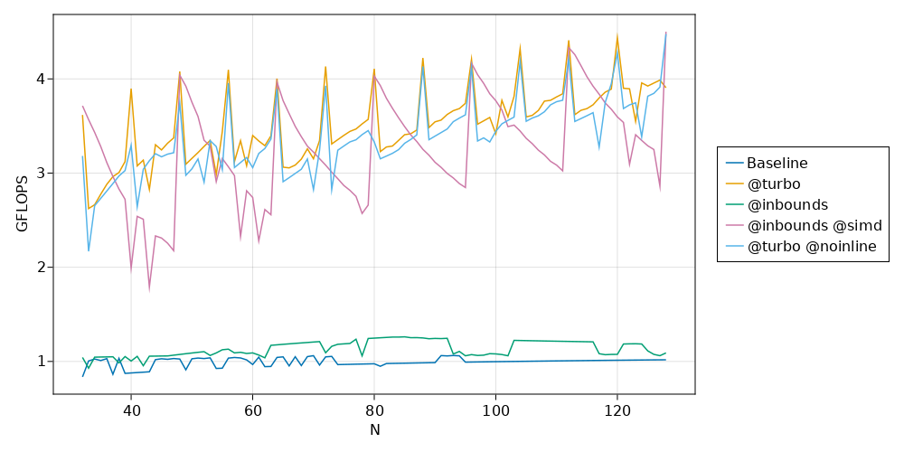
Notice a few things:
As expected, Julia no longer automatically applies
@simdto the@inboundsvariantThe sawtooth is more dramatic for
@inbounds @simd@turboonly beats@simdabout half the time, for this task on on this CPU@turbohas an interesting performance spike for \(N \bmod 8 = 0\)Performance is terrible if some form of SIMD is not applied