Hourly IAM

A simple comparison of IAM calculated at high- and low-resolution.

import pandas as pd
import pvlib
import matplotlib.pyplot as plt

times = pd.date_range('2019-01-01', '2019-12-31', freq='1min', tz='Etc/GMT+5')
location = pvlib.location.Location(40, -80)
solpos = location.get_solarposition(times)
tracker = pvlib.tracking.singleaxis(solpos.apparent_zenith, solpos.azimuth,
                                    gcr=0.5, backtrack=True, axis_azimuth=180)

iam = pvlib.iam.ashrae(tracker.aoi)

# hourly average IAM, i.e. the "true" iam for each hourly interval:
iam_avg = iam.resample('h').mean().reindex(iam.index).ffill()
# hourly sampled IAM, i.e. the iam that PVsyst would calculate:
iam_sample_middle = iam.loc[iam.index.minute == 30]
# the "true average" points on the same index:
iam_avg_middle = iam_avg[iam_avg.index.minute == 30]

plt.figure()
plt.scatter(iam_avg_middle, iam_sample_middle)
plt.plot([0, 1], [0, 1], c='k')
plt.xlabel('Hourly Average')
plt.ylabel('Middle of Interval')

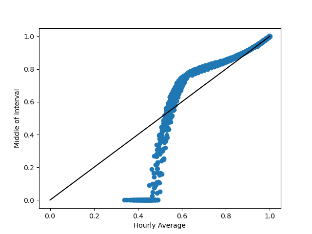
Out:

Text(42.597222222222214, 0.5, 'Middle of Interval')

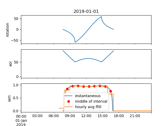
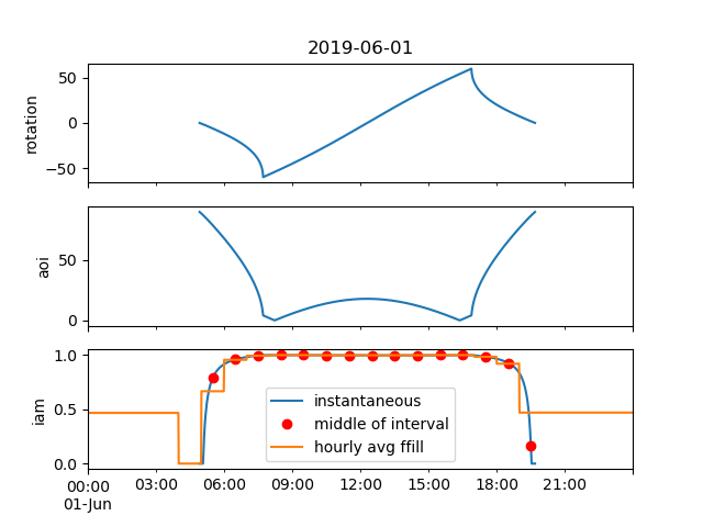
for date in ['2019-01-01', '2019-06-01']:
    fig, axes = plt.subplots(3, 1, sharex=True)
    tracker.tracker_theta.plot(ax=axes[0])
    axes[0].set_ylabel('rotation')

    tracker.aoi.plot(ax=axes[1])
    axes[1].set_ylabel('aoi')

    iam.plot(ax=axes[2], label='instantaneous')
    iam_sample_middle.plot(ax=axes[2], c='red', ls='', marker='o',
                           label='middle of interval')
    iam_avg.plot(ax=axes[2], label='hourly avg ffill')

    axes[2].set_ylabel('iam')
    axes[2].legend()

    idx = iam.loc[date].index
    axes[2].set_xlim(idx[0], idx[-1])
    axes[0].set_title(date)

• 
• 

previous

Tilt Correlation Art

next

Insolation by orientation