Diffuse self-shading

How big a deal is row-to-row diffuse shading?

Most self-shading modeling is (rightly) focused on beam shading, but there is also a reduction in diffuse irradiance caused by a portion of the sky dome being blocked by the row in front. The magnitude of the loss is small compared to typical beam shading losses though, so it doesn’t get much attention.

import pvlib
from pvlib import shading
import pandas as pd
import numpy as np
import matplotlib.pyplot as plt

location = pvlib.location.Location(40, -80, 'US/Eastern')
winter = pd.date_range('2019-01-01', '2019-01-02', freq='5min', tz='US/Eastern')
summer = pd.date_range('2019-06-01', '2019-06-02', freq='5min', tz='US/Eastern')

def get_diffuse_loss(times, gcr, backtrack):
    solar_position = location.get_solarposition(times)
    tracker_data = pvlib.tracking.singleaxis(solar_position.apparent_zenith, solar_position.azimuth,
                                             axis_azimuth=180, gcr=gcr, backtrack=backtrack)

    masking_angle = shading.masking_angle_passias(tracker_data['surface_tilt'], gcr)
    blocked_fraction = shading.sky_diffuse_passias(masking_angle)
    return blocked_fraction * 100

combos = [('Summer', summer), ('Winter', winter)]
fig, axes = plt.subplots(1, 2, sharey=True, figsize=(8, 4))
for i, (title, times) in enumerate(combos):
    get_diffuse_loss(times, 0.4, True).plot(label='backtracking', ax=axes[i])
    get_diffuse_loss(times, 0.4, False).plot(label='true-tracking', ax=axes[i])
    axes[i].set_title(title)
    axes[i].legend(loc='lower center', bbox_to_anchor=(0.5, -0.35), ncol=2)

axes[0].set_ylabel('In-Plane Sky Diffuse Loss [%]')
plt.show()

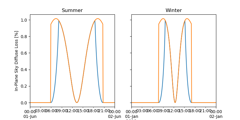
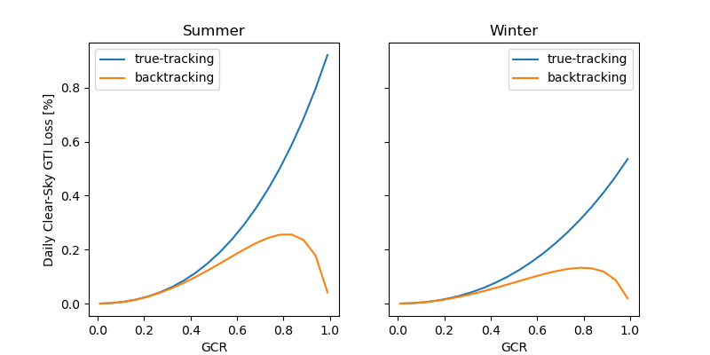
Note that the y-axis there is loss of in-plane sky diffuse irradiance, not total in-plane irradiance. It would be easier to interpret as the loss in total in-plane irradiance. Here’s that daily roll-up loss, this time calculating the loss as fraction of total in-plane irradiance, as a function of GCR:

def avg_loss(times, gcr, backtrack):
    solar_position = location.get_solarposition(times)
    tracker_data = pvlib.tracking.singleaxis(solar_position.apparent_zenith, solar_position.azimuth,
                                             axis_azimuth=180, gcr=gcr, backtrack=backtrack)

    masking_angle = shading.masking_angle_passias(tracker_data['surface_tilt'], gcr)
    blocked_fraction = shading.sky_diffuse_passias(masking_angle)

    cs = location.get_clearsky(times)
    am = location.get_airmass(times)
    dni_et = pvlib.irradiance.get_extra_radiation(times)
    poa_components = pvlib.irradiance.get_total_irradiance(tracker_data.surface_tilt,
                                                           tracker_data.surface_azimuth,
                                                           solar_position.apparent_zenith,
                                                           solar_position.azimuth,
                                                           cs.dni, cs.ghi, cs.dhi,
                                                           dni_extra=dni_et,
                                                           airmass=am['airmass_absolute'], model='haydavies')
    poa_global = poa_components['poa_global']
    poa_reduced = poa_global - blocked_fraction * poa_components['poa_sky_diffuse']
    return (1 - poa_reduced.sum() / poa_global.sum()) * 100

fig, axes = plt.subplots(1, 2, sharey=True, figsize=(8, 4))
for i, (title, times) in enumerate(combos):
    gcrs = np.linspace(0.01, 0.99, 20)
    bt_loss = [avg_loss(times, gcr, True) for gcr in gcrs]
    tt_loss = [avg_loss(times, gcr, False) for gcr in gcrs]

    axes[i].plot(gcrs, tt_loss, label='true-tracking')
    axes[i].plot(gcrs, bt_loss, label='backtracking')
    axes[i].legend()
    axes[i].set_xlabel('GCR')
    axes[i].set_title(title)

axes[0].set_ylabel('Daily Clear-Sky GTI Loss [%]')
plt.show()

# sphinx_gallery_thumbnail_number = 2

previous

Misalignment Error

next

Timestamp Sorting Efficiency