Detailed balance limit

A not-so-precise recreation of the detailed balance limit (or at least the spectral effect).

The detailed balance limit includes the effect of several loss mechanisms in single-junction PV cells. Here we only consider spectral losses, which is probably the biggest effect.

We’ll use SPECTRL2 for a clear-sky spectrum using assumptions from 1.

References

1

Bird, R, and Riordan, C., 1984, “Simple solar spectral model for direct and diffuse irradiance on horizontal and tilted planes at the earth’s surface for cloudless atmospheres”, NREL Technical Report TR-215-2436 doi:10.2172/5986936.

from pvlib import spectrum, solarposition, irradiance, atmosphere
import pandas as pd
import numpy as np
import matplotlib.pyplot as plt

# assumptions from the technical report:
lat = 37
lon = -100
tilt = 37
azimuth = 180
pressure = 101300  # sea level, roughly
water_vapor_content = 0.5  # cm
tau500 = 0.1
ozone = 0.31  # atm-cm
albedo = 0.2

times = pd.date_range('1984-03-20 09:17', freq='h', periods=1, tz='Etc/GMT+7')
solpos = solarposition.get_solarposition(times, lat, lon)
aoi = irradiance.aoi(tilt, azimuth, solpos.apparent_zenith, solpos.azimuth)

# The technical report uses the 'kasten1966' airmass model, but later
# versions of SPECTRL2 use 'kastenyoung1989'.  Here we use 'kasten1966'
# for consistency with the technical report.
relative_airmass = atmosphere.get_relative_airmass(solpos.apparent_zenith,
                                                   model='kasten1966')

spectra = spectrum.spectrl2(
    apparent_zenith=solpos.apparent_zenith,
    aoi=aoi,
    surface_tilt=tilt,
    ground_albedo=albedo,
    surface_pressure=pressure,
    relative_airmass=relative_airmass,
    precipitable_water=water_vapor_content,
    ozone=ozone,
    aerosol_turbidity_500nm=tau500,
)
spectrum = spectra['poa_global'].ravel()
wavelength = spectra['wavelength']

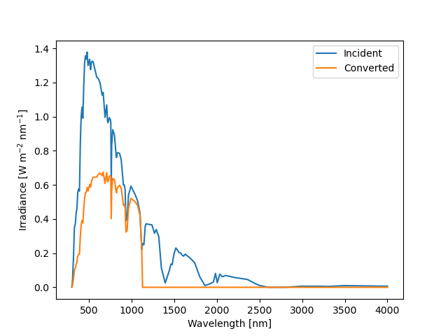
# neglecting constants; they'll cancel out in the end:
flux = spectrum * wavelength

si_bandgap = 1130
si_captured = (flux * (si_bandgap > wavelength)) / si_bandgap

plt.plot(wavelength, spectrum, label='Incident')
plt.plot(wavelength, si_captured, label='Converted')
plt.xlabel('Wavelength [nm]')
plt.ylabel('Irradiance [W m$^{-2}$ nm$^{-1}$]')
plt.legend()
plt.show()

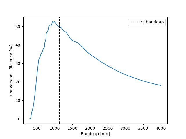
captured_irradiance = [
    (flux * (bandgap > wavelength)).sum() / bandgap
    for bandgap in wavelength
]
plt.plot(wavelength, 100 * (captured_irradiance / spectrum.sum()))
plt.axvline(si_bandgap, c='k', ls='--', label='Si bandgap')
plt.xlabel('Bandgap [nm]')
plt.ylabel('Conversion Efficiency [%]')
plt.legend()
plt.show()

previous

Insolation by orientation

next

Solar Tracking Art