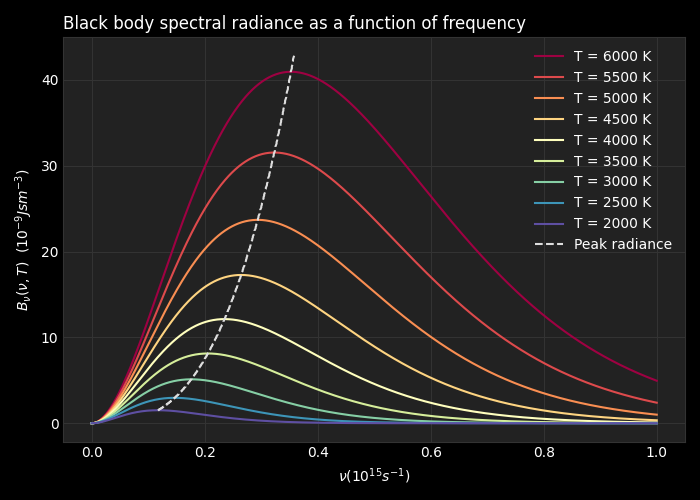
Planck’s Law

Recreating (with matplotlib) the figure in this Bokeh release announcement: https://blog.bokeh.org/bokeh-2-4-6f8a842dfb4f

import numpy as np
import matplotlib.pyplot as plt

plt.style.use('dark_background')
plt.rcParams['mathtext.fontset'] = 'dejavuserif'

h = 6.62607004e-34  # m^2 kg s^-1
k = 1.38064852e-23  # m^2 kg s^-2 K^-1
c = 299792458  # m s^-1


def planck(nu, T):
    return (2*h*nu**3 / c**2) * (np.exp(h*nu/(k*T)) - 1)**-1


def max_planck(nu, T):
    Bv = planck(nu, T)
    return nu[np.argmax(Bv)]


temperatures = np.arange(2000, 6001, 500)[::-1]  # K
frequencies = np.linspace(1, 10**15, 1000)  # Hz
radiances = np.array([planck(frequencies, temperature) for temperature in temperatures])
labels = [f'T = {temperature} K' for temperature in temperatures]
colors = plt.cm.Spectral(np.linspace(0, 1, len(temperatures)))

fig, ax = plt.subplots(figsize=(7, 5))
for radiance, label, color in zip(radiances, labels, colors):
    lines = ax.plot(frequencies/1e15, radiance*1e9, label=label, color=color)

temperature = np.arange(2000, 6100, 10)
max_radiance_frequency = np.array([max_planck(frequencies, T) for T in temperature])
max_radiance = planck(max_radiance_frequency, temperature)
ax.plot(max_radiance_frequency/1e15, max_radiance*1e9, label='Peak radiance', ls='--', c='#DDDDDD')

ax.set_xlabel(r"$\nu (10^{15} s^{-1})$")
ax.set_ylabel(r"$B_\nu (\nu, T)$  $(10^{-9} J s m^{-3})$")
ax.legend(frameon=False)
ax.grid(color='#333333')
ax.set_facecolor('#222222')
ax.set_title('Black body spectral radiance as a function of frequency', loc='left')
plt.setp(ax.spines.values(), color='#333333')
plt.setp([ax.get_xticklines(), ax.get_yticklines()], color='#333333')
ax.tick_params(axis='both', which='both', length=0)

fig.tight_layout()

plt.style.use('default')

previous

Newton Fractals

next

Reflections